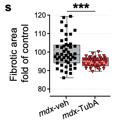
Fig 2s – Pharmacological inhibition of HDAC6 improves muscle phenotypes in dystrophin-deficient mice by downregulating TGF-β via Smad3 acetylation

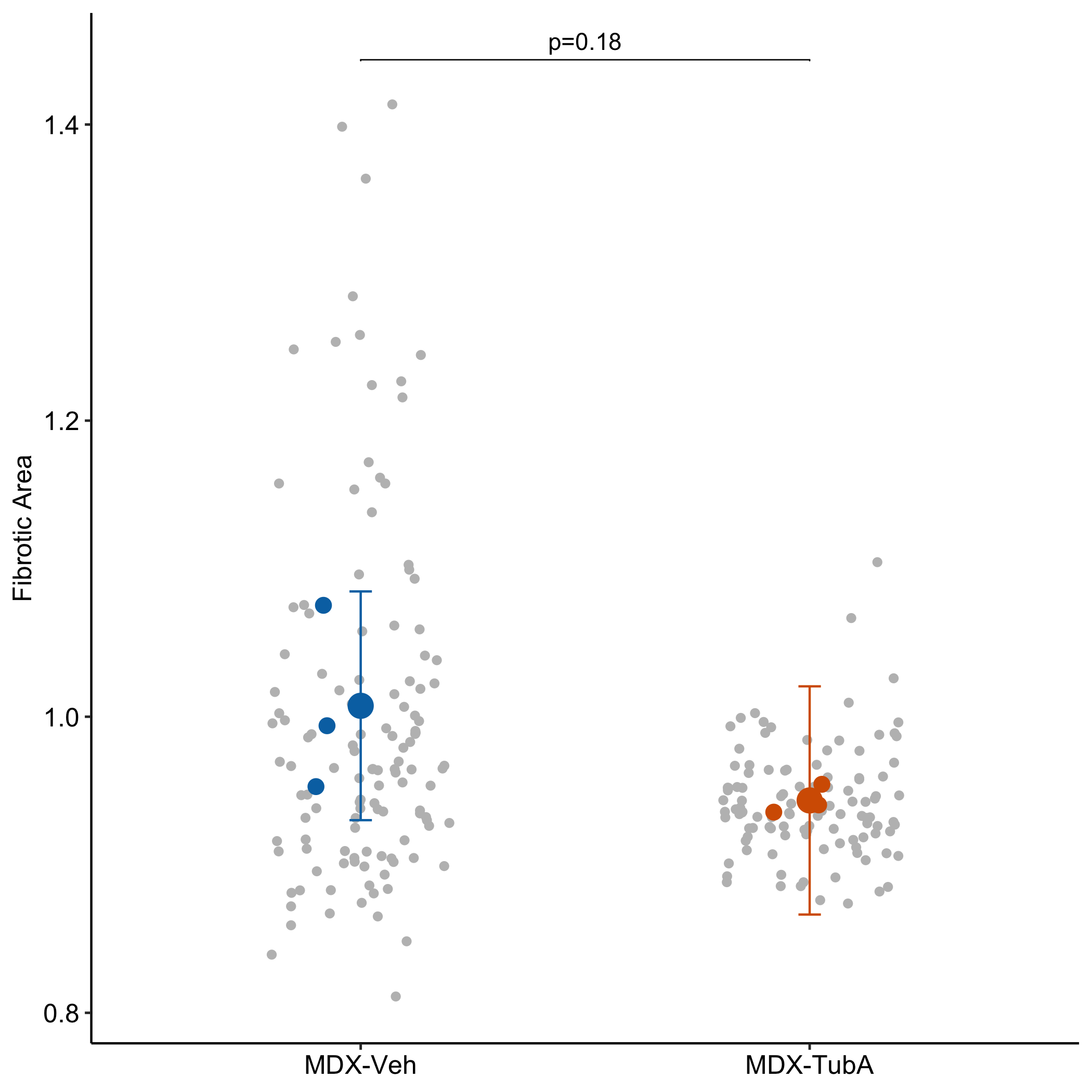
Fig 2s is a Completely Randomized Design with subsampling (CRDS), with 28-49 technical replicates per mouse. The researchers used a Mann-Whitney test that ignored the technical replication. This analysis is massively pseudoreplicated because techanical replicates are not independent evidence of effect of treatment. Individual mouse ID was archived, which makes it easy to re-analyze with models that account for the non-independence. The p-value accounting for non-independence is 0.18 while the p-value using Mann-Whitney on all data is 0.0002. Whoops!
linear mixed model
random intercept
CRDS
nested ANOVA
ggplot
Author

Jeff Walker

Published

June 2, 2024

Modified

October 2, 2024

Fig 2s repro generated using ggplot. The technical replicates are de-emphasized by using a gray color.

Vital info

Data From: Osseni, Alexis, et al. “Pharmacological inhibition of HDAC6 improves muscle phenotypes in dystrophin-deficient mice by downregulating TGF-β via Smad3 acetylation.” Nature Communications 13.1 (2022): 7108.

Fig: 2s download data

key words:

Published methods: Mann-Whitney U on all data

Design: Completely Randomized Design with Subsampling (CRDS)

Response: fibrotic area

Key learning concepts: linear mixed model, random intercept, nested ANOVA

Quick learning explanation: Nested data are measures within a discrete unit or a hierarchy of units, for example technical replicates within a tumor within a mouse.Pseudoreplication is the analysis of subsampled (technical) replicates as if they were independent measures of treatment effects. They aren’t, because technical replicates within a unit (a mouse, a culture) share causes of variation that not shared by technical replicates in other units. This is a violation of the assumption of independence of errors.

More info: Chapter 16 Models for non-independence – linear mixed models

The experiment

Published results

Fig 2s from the article

Setup

Import and Wrangle

Code
data_from <- "Pharmacological inhibition of HDAC6 improves muscle phenotypes in dystrophin-deficient mice by downregulating TGF-β via Smad3 acetylation"
file_name <- "ncomms-source-data files OSSENI et al.xlsx"
file_path <- here(data_folder, data_from, file_name)

fig2s_wide <- read_excel(file_path,
                    sheet = "Figure 2",
                    range = "E138:J186",
                    col_names = FALSE) |>
  data.table()
mouse_id <- paste("mouse", 1:6, sep = "_")
treatment_levels <- c("MDX-Veh", "MDX-TubA")
mouse_treatment <- paste(rep(treatment_levels, each = 3), mouse_id)
colnames(fig2s_wide) <- mouse_treatment
fig2s <- melt(fig2s_wide,
              measure.vars = mouse_treatment,
              variable.name = "mouse_treatment",
              value.name = "fibrotic_area") |>
  na.omit()
fig2s[, c("treatment", "mouse_id") := tstrsplit(mouse_treatment, " ")]
fig2s[, treatment := factor(treatment, levels = treatment_levels)]

file_out_name <- "fig2s-CRDS-Pharmacological inhibition of HDAC6 improves muscle phenotypes in dystrophin-deficient mice by downregulating TGF-β via Smad3 acetylation.xlsx"
fileout_path <- here(data_folder, data_from, file_out_name)
write_xlsx(fig2s, fileout_path)

Fit the models

The Mann-Whitney U test used by the authors

Code
m0 <- wilcox.test(fig2s[treatment == treatment_levels[1], fibrotic_area], fig2s[treatment == treatment_levels[2], fibrotic_area])
m0

    Wilcoxon rank sum test with continuity correction

data:  fig2s[treatment == treatment_levels[1], fibrotic_area] and fig2s[treatment == treatment_levels[2], fibrotic_area]
W = 8740, p-value = 0.000204
alternative hypothesis: true location shift is not equal to 0

A linear mixed-model is the best practice method

Code
m1 <- lmer(fibrotic_area ~ treatment + (1 | mouse_id), data = fig2s)
m1_emm <- emmeans(m1, specs = "treatment")
m1_pairs <- contrast(m1_emm, method = "revpairwise") |>
  summary(infer = TRUE)
m1_pairs
 contrast               estimate     SE df lower.CL upper.CL t.ratio p.value
 (MDX-TubA) - (MDX-Veh)  -0.0639 0.0393  4   -0.173   0.0452  -1.627  0.1792

Degrees-of-freedom method: kenward-roger 
Confidence level used: 0.95 

A nested ANOVA is a classical method that is equivalent to the linear mixed model above when there are an equal number of technical replicates per mouse, but will be close otherwise. In general, things will rarely go wrong if one uses a nested ANOVA instead of the linear mixed-model. GraphPad Prism does nested ANOVA but not a linear mixed model.

Code
m2 <- aov_4(fibrotic_area ~ treatment + (1 | mouse_id), data = fig2s)
m2_emm <- emmeans(m2, specs = "treatment")
m2_pairs <- contrast(m2_emm, method = "revpairwise") |>
  summary(infer = TRUE)
m2_pairs
 contrast               estimate     SE df lower.CL upper.CL t.ratio p.value
 (MDX-TubA) - (MDX-Veh)  -0.0647 0.0395  4   -0.174   0.0449  -1.639  0.1766

Confidence level used: 0.95 

Plotting technical replicates

The technical replicates are de-emphasized by using a gray color. The modeled means of each mouse are colored by treatment (these are the predicted means of the linear mixed model and not the simple mean of each mouse). The model means of each treatment are colord by treatment.

Code
# get estimated means from linear model
fig2s_means <- fig2s[, .(fibrotic_area = mean(fibrotic_area)), by = .(treatment, mouse_id)]
fig2s_means[, fibrotic_area_model := predict(m1, fig2s_means)]
m1_emm_dt <- m1_emm |>
  summary() |>
  data.table()
m1_pairs_dt <- m1_pairs |>
  data.table()
gg <- ggplot(data = fig2s,
             aes(x = treatment,
                 y = fibrotic_area)) +
  # technical reps
  geom_jitter(color = "gray",
              width = 0.2) +
  geom_jitter(data = fig2s_means,
              aes(x = treatment,
                  y = fibrotic_area_model,
                  color = treatment),
              size = 3,
              width = 0.1,
              show.legend = FALSE) +
  # mean and error
  geom_point(data = m1_emm_dt,
             aes(x = treatment,
                 y = emmean,
                 color = treatment),
             size = 5,
             show.legend = FALSE) +
  geom_errorbar(data = m1_emm_dt,
                aes(x = treatment, 
                    y = emmean,
                    ymin = lower.CL, ymax = upper.CL,
                    color = treatment),
                width = 0.05,
                show.legend = FALSE) +
  ylab("Fibrotic Area") +
  scale_color_manual(values = pal_okabe_ito_2) +
  theme_pubr() +
  theme(axis.title.x = element_blank()) +
  NULL

  # add p-values
m1_pairs_dt[, group1 := "MDX-TubA"]
m1_pairs_dt[, group2 := "MDX-Veh"]
m1_pairs_dt[, p := p.value |>
              p_round(digits = 2) |>
              p_format(digits = 2, accuracy = 1e-04, add.p = TRUE)]
maxy <- fig2s[, max(fibrotic_area)]
miny <- fig2s[, min(fibrotic_area)]
m1_pairs_dt[, y.position := maxy + 0.05*(maxy - miny)]

gg <- gg +
  stat_pvalue_manual(
    data = m1_pairs_dt,
    label = "p",
    tip.length = 0.001)

gg

Code
save_it <- FALSE
if(save_it){
out_fig <- "fig2s_ggplot.png"
out_path <- here("figs", data_from, out_fig)
ggsave(out_path)
}